2. The different model classes#
This section will show you the different models implemented in HMP
First we simulate the data by calling the demo function, which is only used for this tutorial.
[1]:
import matplotlib.pyplot as plt
import numpy as np

# Running the demo function in the simulation module
from hmp.simulations import demo

n_events = 5 #how many events are simulated in the demo
# Performing simulation of trials
epoch_data, sim_source_times, info = demo()
Simulating /home/gabriel/ownCloud/projects/RUGUU/hmp/docs/source/notebooks/sample_data/demo_dataset_raw.fif
/home/gabriel/ownCloud/projects/RUGUU/hmp/docs/source/notebooks/sample_data/demo_dataset_raw.fif simulated
Processing participant /home/gabriel/ownCloud/projects/RUGUU/hmp/docs/source/notebooks/sample_data/demo_dataset_raw.fif's raw eeg
We preprocess the data as in Turorial 1 and we want 10 PC components (more on that for the next tutorial on real data):
[2]:
from hmp.transformers import ProjPCA

preprocessed = ProjPCA(epoch_data, n_comp=10, interval_id='rt')
50 positively defined intervalsbetween 0.01 and inf seconds.
Rejection summary:
 0 trials rejected based on threshold of None
 0 trials rejected based on interval limit of (0.01, inf)
 0 trials detected with no interval (e.g. preprocessing or interval exceeding epoch))
And we create a standard template and distribution as in Tutorial 1, this will be used for all the model classes
[3]:
from hmp.patterns import HalfSine
from hmp.trialdata import TrialData

event_properties = HalfSine.create_expected(sfreq=epoch_data.sfreq)
trial_data = TrialData.from_transformer(preprocessed, pattern=event_properties.template)
Model with a fixed number of event with EventModel#
This type of model is the basic model used by HMP. All subsequent ones call this class implicitely. The model works with an a priori number of events defined in the n_events parameter
The EM algorithm (see previous documentation section here) is initiated with the starting point that all events are spread out evenly across the mean reaction time (RT) and that no channels are contributing to the events
[4]:
from hmp.models import EventModel

model_null = EventModel(event_properties, n_events=n_events,
                        max_iteration=0)#max_iteration=0 prevents from actually going through the EM
model_null.fit(trial_data, verbose=False)# Just to illustrate the default starting points
/home/gabriel/ownCloud/projects/RUGUU/hmp/hmp/models/event.py:580: RuntimeWarning: Convergence failed, estimation hit the maximum number of iterations: (0)
  warn(
[5]:
model_null.time_pars
[5]:
array([[[2.        , 5.87166667],
        [2.        , 5.87166667],
        [2.        , 5.87166667],
        [2.        , 5.87166667],
        [2.        , 5.87166667],
        [2.        , 5.87166667]]])
[6]:
model_null.channel_pars
[6]:
array([[[0., 0., 0., 0., 0., 0., 0., 0., 0., 0.],
        [0., 0., 0., 0., 0., 0., 0., 0., 0., 0.],
        [0., 0., 0., 0., 0., 0., 0., 0., 0., 0.],
        [0., 0., 0., 0., 0., 0., 0., 0., 0., 0.],
        [0., 0., 0., 0., 0., 0., 0., 0., 0., 0.]]])
Fit transform#
As seen previously, when fitting an EventModel both the time and channel parameters will get updated depending on the data. The time parameters will be updated to reflect the expected time interval between each event, and the channel parameters will be updated to reflect the expected contribution of each channel to each event.
[7]:
model = EventModel(event_properties, n_events=n_events)

#Fitting
loglikelihood, estimates = model.fit_transform(trial_data)# Fits the model and returns the estimates as event probabilities per sample
Estimating 5 events model with 1 starting point(s)
Combined, these time and channel parameters define the event probabilities for each sample in the data.
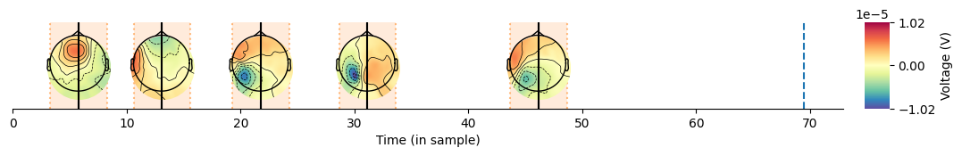
The estimates variable contains these probabilities, which can be visualized using the plot_topo_timecourse function.
[8]:
from hmp.visu import plot_topo_timecourse

#Visualizing
plot_topo_timecourse(epoch_data, estimates, info, magnify=1, sensors=False, times_to_display=None)
plt.vlines(np.mean(np.cumsum(sim_source_times,axis=1),axis=0)[:-1],
           np.repeat(0,n_events), np.repeat(1,n_events), zorder=10, color='k')
[8]:
<matplotlib.collections.LineCollection at 0x7f9f127a55e0>
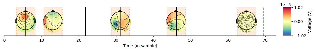
In this case HMP misses the 2nd event, which is not surprising as it is very close to the 1st one. The reason is that the EM algorithm is sensitive to the starting points given to the relative event onsets. By default, the fit method uses the starting point we illustrated above. But we can provide some informed one if we wanted:
Informed starting points#
[9]:
time_parameters = np.array([[[[2.        , 2.5],# Expecting a shorter inter-event duration
                        [2.        , 2.5],# Expecting a shorter inter-event duration
                        [2.        , 2.5],# Expecting a shorter inter-event duration
                        [2.        , 10],# Expecting a longer inter-event duration
                        [2.        , 10],# Expecting a longer inter-event duration
                        [2.        , 10]]]])# Expecting a longer inter-event duration
# Estimating an informed model
ll_informed, estimates_informed = model.fit_transform(trial_data, time_pars=time_parameters)# Providing the informed starting points
Estimating 5 events model
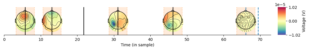
[10]:
#Visualizing
plot_topo_timecourse(epoch_data, estimates_informed, info, magnify=1, sensors=False)
plt.vlines(np.mean(np.cumsum(sim_source_times,axis=1),axis=0)[:-1],
           np.repeat(0,n_events), np.repeat(1,n_events), zorder=10, color='k')
[10]:
<matplotlib.collections.LineCollection at 0x7f9f10d12c30>

Hooray, the 2nd event is now found! The reason is that the starting points are now more appropriate for the data. However, this is not always possible to know in advance, so we will now look at how to use random starting points.
Random starting points#
Here we will just generate random time parameters to avoid leaving parameter space unexplored.
[11]:
model_random = EventModel(event_properties, n_events=n_events,
                        starting_points=50, max_scale=trial_data.durations.max())
ll_random, estimates_random = model_random.fit_transform(trial_data, cpus=2, )

#Visualizing
plot_topo_timecourse(epoch_data, estimates_random, info, magnify=1, sensors=False)
plt.vlines(np.mean(np.cumsum(sim_source_times,axis=1),axis=0)[:-1],
           np.repeat(0,n_events), np.repeat(1,n_events), zorder=10, color='k')
Estimating 5 events model with 50 starting point(s)
/usr/lib/python3.12/multiprocessing/popen_fork.py:66: DeprecationWarning: This process (pid=27547) is multi-threaded, use of fork() may lead to deadlocks in the child.
  self.pid = os.fork()
[11]:
<matplotlib.collections.LineCollection at 0x7f9f74d2bb00>
Provided enough starting point the method will find the correct solution, here 50 might not be enough, you can try by running this cell again. In any case random starting points are not always the best solution, especially when the number of events is high or if the duration you model (e.g. RT) is very long. In that case, we can use the eliminative or cumulative estimation methods.
Eliminative method#
Another solution is to first estimate a model with the maximal number of possible events that fit in RTs (referred to as ‘the maximal model’), and then decrease the number of events one by one.
The idea is that genuine events will necessarily be found at the expected locations in the maximal model. Because the backward estimation method iteratively removes the weakest event (in terms of likelihood), only the ‘strongest’ events remain even if their location would have been hard to find with a single fit and default starting values.
In order to do this we will use the EliminativeMethod. This function first estimates the maximal number of event (defined based on the event width and the minimum reaction time) using an EventModel, then estimates the max_event - 1 solution by iteratively removing one of the events and picking the solution with the highest likelihood (for more details see Borst & Anderson, 2021) and repeat this until the 1 event
solution is reached.
Default behavior#
[12]:
from hmp.models import EliminativeMethod

elim_model = EliminativeMethod(event_properties)
ll_elim, estimates_elim = elim_model.fit_transform(trial_data)
Estimating all solutions for maximal number of events (10)
Estimating all solutions for 9 events
Estimating all solutions for 8 events
Estimating all solutions for 7 events
Estimating all solutions for 6 events
Estimating all solutions for 5 events
Estimating all solutions for 4 events
Estimating all solutions for 3 events
Estimating all solutions for 2 events
Estimating all solutions for 1 events
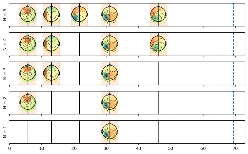
Here we plot the resulting solutions going from the maximal possible number of events (here 9 given the simulated average RT) all the way to a single event.
[13]:
fig, axes = plt.subplots(len(estimates_elim.n_events), 1, figsize=(8, len(estimates_elim.n_events)), sharex=True)
for ax, n_event in zip(axes, estimates_elim.n_events):
    plot_topo_timecourse(epoch_data, estimates_elim.sel(n_events=n_event), info, sensors=False, magnify=1, ax=ax, colorbar=False)
    ax.vlines(np.mean(np.cumsum(sim_source_times, axis=1), axis=0)[:-1],
              np.repeat(0, n_events), np.repeat(1, n_events), zorder=10, color='k')
    ax.set_ylabel(f"N = {n_event.values}")
plt.tight_layout()
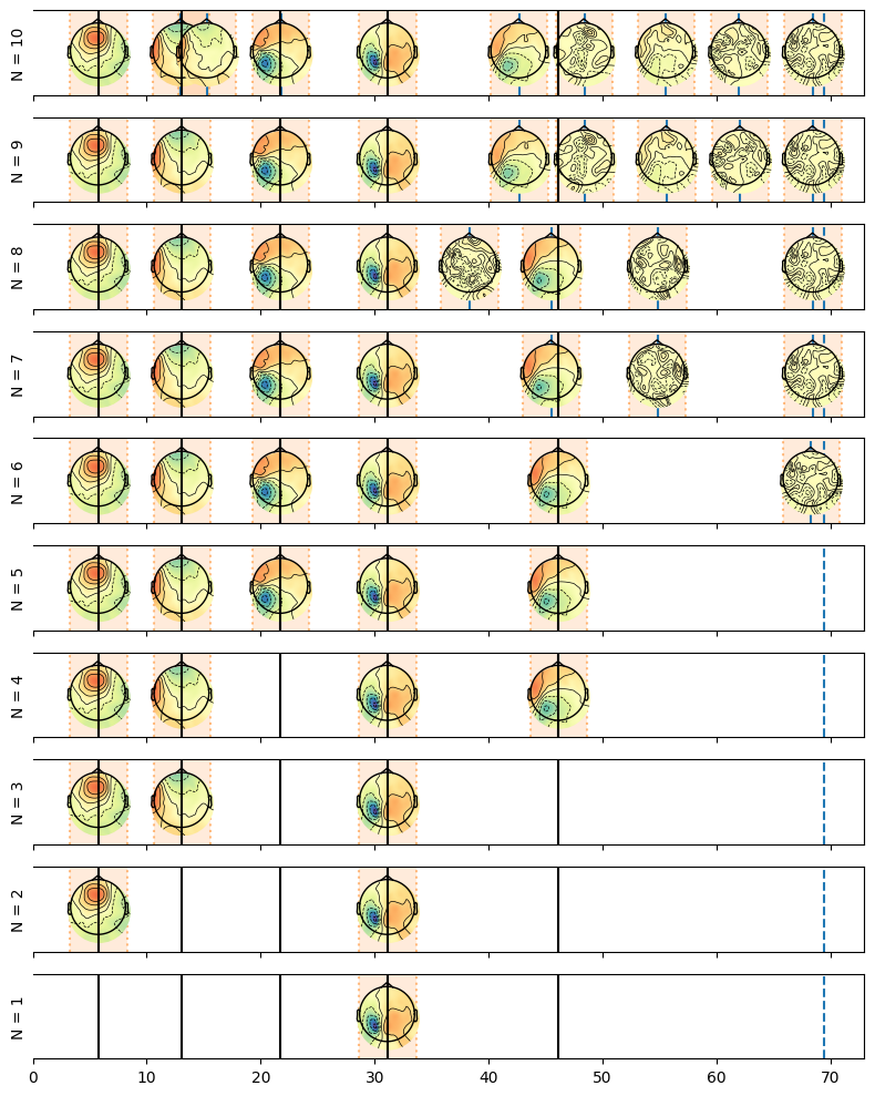
We can see that the maximal model contains the true topograpies and also some false alarms as we requested too many events compared to the true ones. We see that at each removal one of these false alarm gets removed.
From the solutions of the backward estimation we can select the number of events we originally wanted to estimate.
[14]:
selected = estimates_elim.sel(n_events=n_events)
plot_topo_timecourse(epoch_data, selected, info, sensors=False)
plt.vlines(np.mean(np.cumsum(sim_source_times,axis=1),axis=0)[:-1],
           np.repeat(0,n_events), np.repeat(1,n_events), zorder=10, color='k')
[14]:
<matplotlib.collections.LineCollection at 0x7f9f221dfef0>
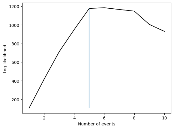
Note however that this is not the maximum likelihood solution, in fact in this example if we look at the log-likelihood of the different solutions we can see that the maximum likelihood solution is actually the 6 events solution as seen in the plot below. The likelihood is evolving in a complex manner with the number of events. On the one hand adding events tends to increase the likelihood, on the other hand if events start to compete for samples (see the maximum model where the third event is split in two), the likelihood can decrease. This is why we can see that the likelihood is not monotonically increasing with the number of events.
[15]:
n_events_backward = [elim_model.submodels[i].n_events for i in elim_model.submodels]
plt.plot(n_events_backward, ll_elim, 'k')
plt.vlines(n_events, np.min(ll_elim), np.max(ll_elim))
plt.xlabel('Number of events')
plt.ylabel('Log-likelihood')
[15]:
Text(0, 0.5, 'Log-likelihood')
Providing a custom maximum model#
Instead of re-estimating a model with a maximum bumber of events we can provide a custom maximum model. This is useful if we know that the maximum number of events is lower than the one estimated by the EliminativeMethod class or if we want to depart from a specific model. In this case, we can provide a custom EventModel to the EliminativeMethod class and start the elimination from there.
[16]:
elim_model_custom = EliminativeMethod(event_properties,  base_fit=model)
ll_elim_custom, estimates_elim_custom = elim_model_custom.fit_transform(trial_data)#Here we use the `model` we fitted above as the base model
Estimating all solutions for 4 events
Estimating all solutions for 3 events
Estimating all solutions for 2 events
Estimating all solutions for 1 events
[17]:
fig, axes = plt.subplots(len(estimates_elim_custom.n_events), 1, figsize=(8, len(estimates_elim_custom.n_events)), sharex=True)
for ax, n_event in zip(axes, estimates_elim_custom.n_events):
    plot_topo_timecourse(epoch_data, estimates_elim_custom.sel(n_events=n_event), info, sensors=False, magnify=1, ax=ax, colorbar=False)
    ax.vlines(np.mean(np.cumsum(sim_source_times, axis=1), axis=0)[:-1],
              np.repeat(0, n_events), np.repeat(1, n_events), zorder=10, color='k')
    ax.set_ylabel(f"N = {n_event.values}")
plt.tight_layout()
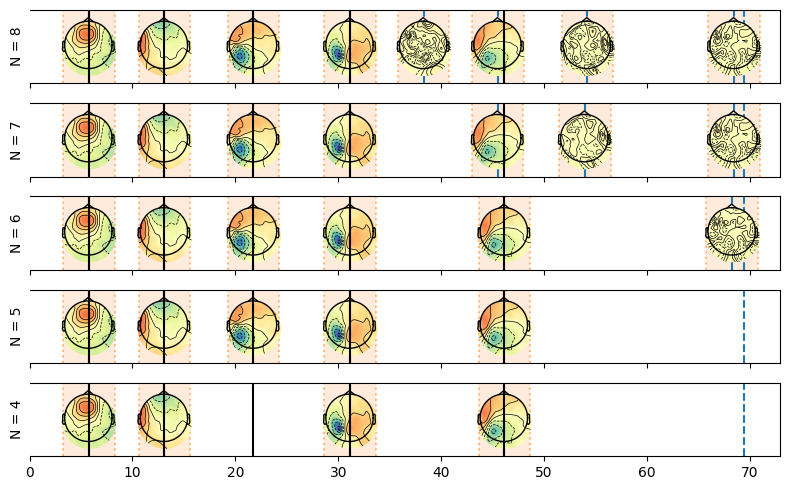
Define a range#
Alternatively we can also specify a range if we don’t want to fully explore all solutions:
[18]:
elim_model_range = EliminativeMethod(event_properties, max_events=8, min_events=3)
ll_range, estimates_range = elim_model_range.fit_transform(trial_data)
Estimating all solutions for maximal number of events (8)
Estimating all solutions for 7 events
Estimating all solutions for 6 events
Estimating all solutions for 5 events
Estimating all solutions for 4 events
[19]:
fig, axes = plt.subplots(len(estimates_range.n_events), 1, figsize=(8, len(estimates_range.n_events)), sharex=True)
for ax, n_event in zip(axes, estimates_range.n_events):
    plot_topo_timecourse(epoch_data, estimates_range.sel(n_events=n_event), info, sensors=False, magnify=1, ax=ax, colorbar=False)
    ax.vlines(np.mean(np.cumsum(sim_source_times, axis=1), axis=0)[:-1],
              np.repeat(0, n_events), np.repeat(1, n_events), zorder=10, color='k')
    ax.set_ylabel(f"N = {n_event.values}")
plt.tight_layout()
Cumulative event fit#
Instead of fitting an n event model this method starts by fitting a 1 event model using each sample from the time 0 (stimulus onset) to the mean RT. Therefore it tests for the landing point of the expectation maximization algorithm given each sample as starting point and the likelihood associated with this landing point. As soon as a starting points reaches the convergence criterion, the function fits an n+1 event model and uses the next samples in the RT for the following event, etc.
[20]:
from hmp.models import CumulativeMethod
Default behavior#
[21]:
model_cumulative = CumulativeMethod(event_properties)
ll_cumulative, estimates_cumulative = model_cumulative.fit_transform(trial_data)
1 events found around times [60]
2 events found around times [60, 140]
3 events found around times [60, 130, 230]
4 events found around times [60, 130, 220, 320]
5 events found around times [60, 130, 220, 320, 460]
Found 5 events
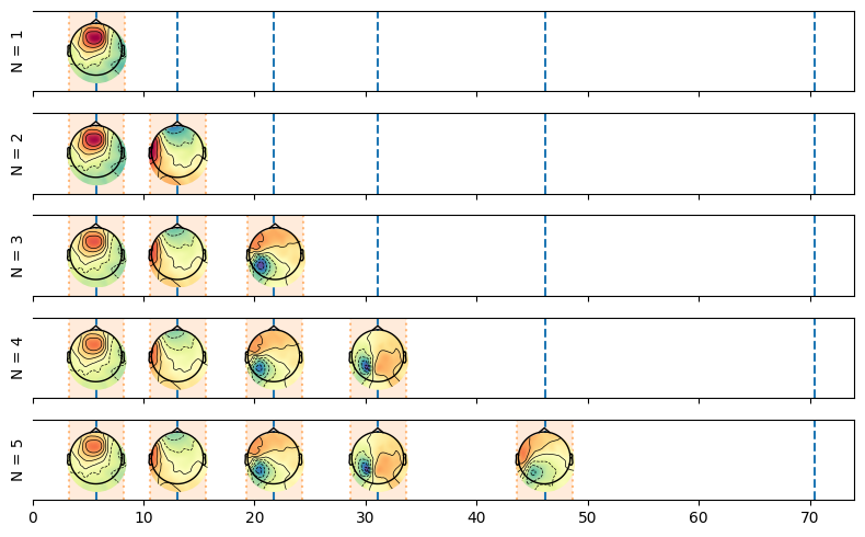
The following cell displays what happened when we fitted the model, as you can see the model iteratively adds events to the model, starting with the one event and a proposal at the first sample, after this event reached a local maxima, the algorithm adds another event just after until convergence, etc. Any additional event that decreases likelihood gets rejected.
[22]:
fig, axes = plt.subplots(len(model_cumulative.submodels), 1, figsize=(8, len(model_cumulative.submodels)), sharex=True)

for ax, model_i in zip(axes, model_cumulative.submodels):
    lkh_i, estimates_i = model_i.transform(trial_data)
    plot_topo_timecourse(epoch_data, estimates_i, info,
                        times_to_display=np.mean(np.cumsum(sim_source_times, axis=1), axis=0),
                        magnify=1, ax=ax, colorbar=False)
    ax.set_ylabel(f"N = {model_i.n_events}")
plt.tight_layout()
We can look how the likelihood unfolded.
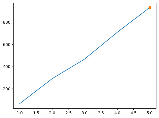
[23]:
cumulative_res = np.array([np.array([x.n_events, x.lkhs[0]]) for x in model_cumulative.submodels])
plt.plot(cumulative_res[:,0], cumulative_res[:,1])
plt.plot(model_cumulative.submodels[-1].n_events, model_cumulative.submodels[-1].lkhs, 'o', label='Fitted model likelihood')
[23]:
[<matplotlib.lines.Line2D at 0x7f9f20f58080>]