4. Advanced - grouping models

[!WARNING] This tutorial and the associated functions are still under construction, only use these functions for development puprose

For this tutorial we will simulate data for two participants, one with noise and one without. We make the simulation deterministic by providing the exact times at which we want the events to occur for two trials. Importantly we will use the same source names and parameters for both participants, but we will swap the first two sources between the two participants. This will allow us to test the grouping model’s ability to handle different event configuration across conditions or participants.

import os.path as op

import matplotlib.pyplot as plt
import numpy as np

import hmp
from hmp import simulations

sfreq = 100
n_events = 3
# Data creation/reading
## Simulation parameters
n_trials = 2
# Times (in milliseconds) for participant A: 3 events per trial, 2 trials with the following time structure:
# On trial 1 the events will occur at 100ms, 300ms, and 400ms after the simulated trial onset
# On trial 2 all inter-event duration were doubled and thus occur at 200ms, 600ms, and 800ms after the simulated trial onset
times = np.array([[100, 200, 100, 100],
                    [200, 400, 200, 200]], dtype='float64')
# Thus, on average, the events appear at 150, 450 and 600ms after trial onset
avg_times = np.cumsum(times.mean(axis=0))[:-1]

# Define source names and parameters, the same for both participants
names_a = ['bankssts-rh', 'bankssts-lh', 'caudalanteriorcingulate-rh', 'bankssts-lh']
# same but the two first sources are swapped
names_b = ['bankssts-lh', 'bankssts-rh','caudalanteriorcingulate-rh', 'bankssts-lh']
sources_a, sources_b = [], []
for name_a_i, name_b_i in zip(names_a, names_b):
    sources_a.append([name_a_i, 10., 4e-8])
    sources_b.append([name_b_i, 10., 4e-8])

## Now we simulated two datasets with the exact same structure except one is noise, one isn't
# Participant A is noisy
files_a = simulations.simulate(sources_a, n_trials, 1, 'dataset_a_raw', overwrite=True,
    sfreq=sfreq, times=times, noise=True, seed=1, path=op.join('sample_data', 'simulated'))
# Participant B has no noise
files_b = simulations.simulate(sources_b, n_trials, 1, 'dataset_b_raw', overwrite=True,
    sfreq=sfreq, times=times, noise=False, seed=1, path=op.join('sample_data', 'simulated'))

Simulating /home/gabriel/ownCloud/projects/RUGUU/hmp/docs/source/notebooks/sample_data/simulated/dataset_a_raw_raw.fif
/home/gabriel/ownCloud/projects/RUGUU/hmp/docs/source/notebooks/sample_data/simulated/dataset_a_raw_raw.fif simulated
Simulating /home/gabriel/ownCloud/projects/RUGUU/hmp/docs/source/notebooks/sample_data/simulated/dataset_b_raw_raw.fif
/home/gabriel/ownCloud/projects/RUGUU/hmp/docs/source/notebooks/sample_data/simulated/dataset_b_raw_raw.fif simulated

Next we read the data as we do for simulations (Tutorial 1)

event_id = {'stimulus':1}#trigger 1 = stimulus
resp_id = {'response':5}
raws, events = [], []
for files in [files_a, files_b]:
    raws.append(files[0])
    events.append(np.load(files[1]))
event_a, event_b = events[0], events[1]

# Data reading
epoch_data = hmp.io.read_mne_data(raws, event_id=event_id, resp_id=resp_id, sfreq=sfreq,
        events_provided=events, verbose=False, subj_name=['a','b'])
positions = simulations.positions()
epoch_data

Processing participant /home/gabriel/ownCloud/projects/RUGUU/hmp/docs/source/notebooks/sample_data/simulated/dataset_a_raw_raw.fif's raw eeg
Processing participant /home/gabriel/ownCloud/projects/RUGUU/hmp/docs/source/notebooks/sample_data/simulated/dataset_b_raw_raw.fif's raw eeg

<xarray.Dataset> Size: 498kB
Dimensions:      (participant: 2, epoch: 2, channel: 59, sample: 521)
Coordinates:
  * epoch        (epoch) int64 16B 0 1
  * channel      (channel) <U7 2kB 'EEG 001' 'EEG 002' ... 'EEG 059' 'EEG 060'
  * sample       (sample) int64 4kB -20 -19 -18 -17 -16 ... 496 497 498 499 500
    event_name   (epoch) object 16B 'stimulus' 'stimulus'
    rt           (epoch) float64 16B 0.5 1.0
  * participant  (participant) <U1 8B 'a' 'b'
Data variables:
    data         (participant, epoch, channel, sample) float32 492kB 7.267e-0...
Attributes:
    sfreq:      100.0
    lowpass:    40.0
    highpass:   0.10000000149011612
    reference:  None
    n_trials:   4
    tmin:       -0.2
    tmax:       5

xarray.Dataset

• Dimensions:
  • participant: 2
  • epoch: 2
  • channel: 59
  • sample: 521
• Coordinates: (6)
  • epoch
    (epoch)
    int64
    0 1

    array([0, 1])

  • channel
    (channel)
    <U7
    'EEG 001' 'EEG 002' ... 'EEG 060'

    array(['EEG 001', 'EEG 002', 'EEG 003', 'EEG 004', 'EEG 005', 'EEG 006',
           'EEG 007', 'EEG 008', 'EEG 009', 'EEG 010', 'EEG 011', 'EEG 012',
           'EEG 013', 'EEG 014', 'EEG 015', 'EEG 016', 'EEG 017', 'EEG 018',
           'EEG 019', 'EEG 020', 'EEG 021', 'EEG 022', 'EEG 023', 'EEG 024',
           'EEG 025', 'EEG 026', 'EEG 027', 'EEG 028', 'EEG 029', 'EEG 030',
           'EEG 031', 'EEG 032', 'EEG 033', 'EEG 034', 'EEG 035', 'EEG 036',
           'EEG 037', 'EEG 038', 'EEG 039', 'EEG 040', 'EEG 041', 'EEG 042',
           'EEG 043', 'EEG 044', 'EEG 045', 'EEG 046', 'EEG 047', 'EEG 048',
           'EEG 049', 'EEG 050', 'EEG 051', 'EEG 052', 'EEG 054', 'EEG 055',
           'EEG 056', 'EEG 057', 'EEG 058', 'EEG 059', 'EEG 060'], dtype='<U7')

  • sample
    (sample)
    int64
    -20 -19 -18 -17 ... 497 498 499 500

    array([-20, -19, -18, ..., 498, 499, 500], shape=(521,))

  • event_name
    (epoch)
    object
    'stimulus' 'stimulus'

    array(['stimulus', 'stimulus'], dtype=object)

  • rt
    (epoch)
    float64
    0.5 1.0

    array([0.5, 1. ])

  • participant
    (participant)
    <U1
    'a' 'b'

    array(['a', 'b'], dtype='<U1')

• Data variables: (1)
  • data
    (participant, epoch, channel, sample)
    float32
    7.267e-07 2.814e-06 ... 3.102e-20

    array([[[[ 7.2670230e-07,  2.8139011e-06,  2.4494673e-06, ...,
              -2.8173332e-07,  6.1022966e-08,  1.9458517e-07],
             [-7.7176361e-07, -1.1794511e-06, -8.6143126e-07, ...,
              -6.5960755e-08,  2.5585692e-07, -1.1207829e-06],
             [-1.6203512e-06, -1.7958705e-06, -1.5639465e-06, ...,
              -1.2660061e-06, -6.1507893e-07, -2.6686470e-07],
             ...,
             [-1.6272576e-06, -2.1308244e-06,  6.5575495e-07, ...,
              -1.2406518e-06, -9.0725493e-08,  4.9919043e-07],
             [-1.8162955e-06, -1.4450530e-06, -6.8021035e-07, ...,
              -1.2480682e-06, -1.1669947e-06, -5.8359467e-07],
             [ 4.2238227e-07,  1.5417423e-07, -2.9267580e-06, ...,
              -2.1300416e-06, -1.8129450e-06, -1.0681758e-06]],
    
            [[-1.8936757e-06, -1.3888381e-06,  9.5652290e-08, ...,
              -1.7150278e-07, -1.1639389e-06, -1.8656847e-06],
             [-1.8611643e-06, -1.2394341e-06, -6.0073489e-07, ...,
              -4.4514613e-06, -4.8433931e-06, -3.2907062e-06],
             [ 1.5535306e-06,  2.2788411e-06,  2.5317838e-06, ...,
              -4.7976249e-07, -3.9611444e-07, -1.5672579e-07],
    ...
               2.4871053e-20,  2.4871053e-20,  2.4871053e-20],
             [ 2.3394156e-20,  2.3394156e-20,  2.3394156e-20, ...,
               2.3394156e-20,  2.3394156e-20,  2.3394156e-20],
             [ 3.1016488e-20,  3.1016488e-20,  3.1016488e-20, ...,
               3.1016488e-20,  3.1016488e-20,  3.1016488e-20]],
    
            [[-4.5222118e-21, -4.5222118e-21, -4.5222118e-21, ...,
              -4.5222118e-21, -4.5222118e-21, -4.5222118e-21],
             [-1.9333354e-21, -1.9333354e-21, -1.9333354e-21, ...,
              -1.9333354e-21, -1.9333354e-21, -1.9333354e-21],
             [ 1.3748756e-21,  1.3748756e-21,  1.3748756e-21, ...,
               1.3748756e-21,  1.3748756e-21,  1.3748756e-21],
             ...,
             [ 2.4871053e-20,  2.4871053e-20,  2.4871053e-20, ...,
               2.4871053e-20,  2.4871053e-20,  2.4871053e-20],
             [ 2.3394156e-20,  2.3394156e-20,  2.3394156e-20, ...,
               2.3394156e-20,  2.3394156e-20,  2.3394156e-20],
             [ 3.1016488e-20,  3.1016488e-20,  3.1016488e-20, ...,
               3.1016488e-20,  3.1016488e-20,  3.1016488e-20]]]],
          shape=(2, 2, 59, 521), dtype=float32)

• Indexes: (4)
  • epoch
    PandasIndex

    PandasIndex(Index([0, 1], dtype='int64', name='epoch'))

  • channel
    PandasIndex

    PandasIndex(Index(['EEG 001', 'EEG 002', 'EEG 003', 'EEG 004', 'EEG 005', 'EEG 006',
           'EEG 007', 'EEG 008', 'EEG 009', 'EEG 010', 'EEG 011', 'EEG 012',
           'EEG 013', 'EEG 014', 'EEG 015', 'EEG 016', 'EEG 017', 'EEG 018',
           'EEG 019', 'EEG 020', 'EEG 021', 'EEG 022', 'EEG 023', 'EEG 024',
           'EEG 025', 'EEG 026', 'EEG 027', 'EEG 028', 'EEG 029', 'EEG 030',
           'EEG 031', 'EEG 032', 'EEG 033', 'EEG 034', 'EEG 035', 'EEG 036',
           'EEG 037', 'EEG 038', 'EEG 039', 'EEG 040', 'EEG 041', 'EEG 042',
           'EEG 043', 'EEG 044', 'EEG 045', 'EEG 046', 'EEG 047', 'EEG 048',
           'EEG 049', 'EEG 050', 'EEG 051', 'EEG 052', 'EEG 054', 'EEG 055',
           'EEG 056', 'EEG 057', 'EEG 058', 'EEG 059', 'EEG 060'],
          dtype='object', name='channel'))

  • sample
    PandasIndex

    PandasIndex(Index([-20, -19, -18, -17, -16, -15, -14, -13, -12, -11,
           ...
           491, 492, 493, 494, 495, 496, 497, 498, 499, 500],
          dtype='int64', name='sample', length=521))

  • participant
    PandasIndex

    PandasIndex(Index(['a', 'b'], dtype='object', name='participant'))

• Attributes: (7)

  sfreq :

  100.0

  lowpass :

  40.0

  highpass :

  0.10000000149011612

  reference :

  None

  n_trials :

  4

  tmin :

  -0.2

  tmax :

  5

Next we preprocess the data and split conditions (or participants in this case). We will use the hmp.preprocessing.Standard class to handle the data preprocessing. We will also create a template for the event properties that we expect in our data.

# Preprocess the data for both participants using the Preprocessing class
hmp_data = hmp.transformers.ProjPCA(epoch_data, n_comp=10)

# Create event property template
event_properties = hmp.patterns.HalfSine.create_expected(sfreq=epoch_data.sfreq)

# Select data for each participant
hmp_data_a = hmp.utils.participant_selection(hmp_data.data, 'a')
hmp_data_b = hmp.utils.participant_selection(hmp_data.data, 'b')

# Create TrialData objects for all data and for each participant
trial_data = hmp.trialdata.TrialData.from_transformer(hmp_data, pattern=event_properties.template)
trial_data_a = hmp.trialdata.TrialData.from_transformer(hmp_data_a, pattern=event_properties.template)
trial_data_b = hmp.trialdata.TrialData.from_transformer(hmp_data_b, pattern=event_properties.template)

4 intervals between 0.01 and inf seconds.
Rejection summary:
 0 trials rejected based on threshold of None
 0 trials rejected based on interval limit of (0.01, inf)
 0 trials detected with no interval (e.g. preprocessing or interval exceeding epoch))

Here we illustrate the ground truth estimates for the events in the noisy data. We will use these to compare the estimates obtained from the different model.

model = hmp.models.EventModel(event_properties, n_events=n_events)
# Recover generating parameters
sim_source_times, true_time_pars, true_channel_pars, _ = \
    simulations.simulated_times_and_parameters(event_a, model, trial_data_a)
# Fixing true parameter in model
model.time_pars = np.array([true_time_pars])
model.channel_pars = np.array([true_channel_pars])
# Ground truth
true_loglikelihood, true_estimates = model.transform(trial_data_a)
hmp.visu.plot_topo_timecourse(epoch_data, true_estimates, positions, as_time=True, colorbar=False)
plt.vlines(avg_times, 0, 1, 'k')

<matplotlib.collections.LineCollection at 0x70789023c9b0>

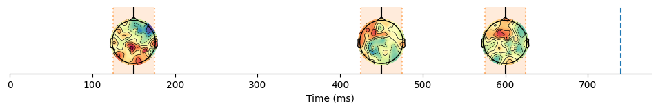
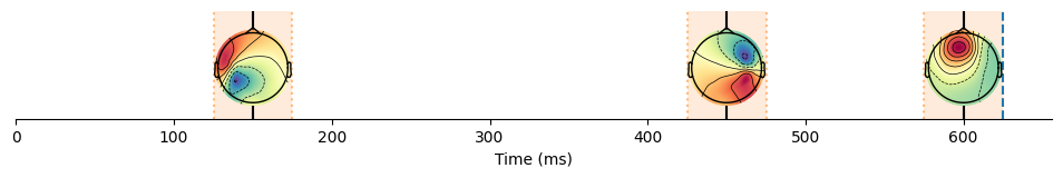
As can be seen the true model estimates the events at the correct time but the topographies are mainly dominated by noise because we only have two trials and the sources have a very low amplitude, thus the SNR is close to zero. Fitting the model on B however gives us the a perfect representation as it is noiseless. Based on this we can see that the last event of the noiseless B estimation is the cleaner version of the last event in A. With a bit of abstraction we can also see that the two first events between A and B are indeed reversed as we requested in the simulation.

model = hmp.models.EventModel(event_properties, n_events=n_events)

# Fit and transform on noiseless B
lkh_b, estimates_b = model.fit_transform(trial_data_b)
hmp.visu.plot_topo_timecourse(epoch_data, estimates_b, positions, as_time=True, colorbar=False)
plt.vlines(avg_times, 0, 1, 'k')

Estimating 3 events model with 1 starting point(s)

<matplotlib.collections.LineCollection at 0x707890183f50>

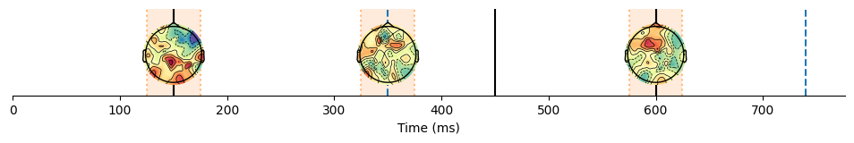
If we first try to fit the model on A the estimates will be dominated by noise. This is because the model is not able to estimate the parameters correctly from the noisy data alone.

model = hmp.models.EventModel(event_properties, n_events=n_events)

# Fit and transform on noisy A
lkh_a, estimates_a = model.fit_transform(trial_data_a)
hmp.visu.plot_topo_timecourse(epoch_data, estimates_a, positions, as_time=True, colorbar=False)
plt.vlines(avg_times, 0, 1, 'k')

Estimating 3 events model with 1 starting point(s)

<matplotlib.collections.LineCollection at 0x70788fd8c8f0>

Fit / transform

A first way to split conditions and use the information from one condition to estimate the other is to use the fit/transform architecture. In this example we can then fit the model to the data of B (noiseless) and transform the data of A using the parameters estimated on B:

model = hmp.models.EventModel(event_properties, n_events=n_events)

# Fit on noiseless B
model.fit(trial_data_b)
# Transform on noisy A
lkh_a_transform, estimates_a_transform = model.transform(trial_data_a)
hmp.visu.plot_topo_timecourse(epoch_data, estimates_a_transform, positions, as_time=True, colorbar=False)
plt.vlines(avg_times, 0, 1, 'k')

Estimating 3 events model with 1 starting point(s)

<matplotlib.collections.LineCollection at 0x7078902ef560>

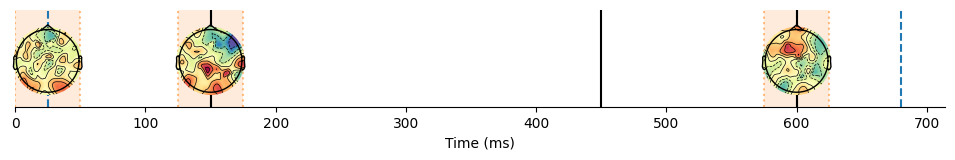
In this case this turns out pretty bad because we estimate the two first events based on B while they are reversed in A. Thus the estimation of the channel_pars parameters does not help to correclty estimate the model in A, to the contrary doing so will actually make the estimates worse than if we had not used the parameters from B at all.

Grouping models

HMP implements grouping models, models that share time and channel parameters across groups (e.g. condition or participant) based on a map. This map is a 2D array where each row corresponds to a level and each column corresponds to an expected event (Note we need to know how many events are present to write the map, thus this only works on theEventModel class).

The values in the map indicate which sources are shared across participants. As a wrong example we could estimate a grouping where all the parameters for each event are shared across the two groups A and B.

# testing grouping model with all parameters shared across participants
channel_map = np.array([[0, 0, 0],    # All events share the same channel parameters
                        [0, 0, 0]])
time_map = np.array([[0, 0, 0, 0],    # All events share the same time parameters
                     [0, 0, 0, 0]])
grouping_dict = {'participant': ['a', 'b']}  # Define participant groups

# Fit the multilevel model with shared parameters and get estimates
lkh_comb, estimates_comb = model.fit_transform(
    trial_data,
    time_map=time_map,
    channel_map=channel_map,
    grouping_dict=grouping_dict
)

group "participant" analyzed, with groups: ['a', 'b']

Coded as follows:
0: ['a']
1: ['b']

Channel map:
0:  [0 0 0]
1:  [0 0 0]

Time map:
0:  [0 0 0 0]
1:  [0 0 0 0]
Estimating 3 events model with 1 starting point(s)

hmp.visu.plot_topo_timecourse(epoch_data, estimates_comb, positions, as_time=True, colorbar=False, magnify=0.75, )
plt.vlines(avg_times,0,2, 'k')

<matplotlib.collections.LineCollection at 0x707895a0bcb0>

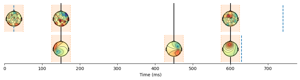
In this case, we expect that the parameters are all shared, thus, the first event in A is moved to the second event of B as the first event in B is the second event in A.

Instead we can inform the model that we expect different topographies for the first two events

# testing grouping model with all parameters shared across participants
channel_map = np.array([[0, 0, 0],   # The two first events are not shared and will be estimated separatebly for both B and A
                        [1, 1, 0]])
time_map = np.array([[0, 0, 0, 0],    # All events still share the same time parameters
                     [0, 0, 0, 0]])
grouping_dict = {'participant': ['a', 'b']}  # Define participant groups

# Fit the multilevel model with shared parameters and get estimates
lkh_comb, estimates_comb = model.fit_transform(
    trial_data,
    time_map=time_map,
    channel_map=channel_map,
    grouping_dict=grouping_dict
)

group "participant" analyzed, with groups: ['a', 'b']

Coded as follows:
0: ['a']
1: ['b']

Channel map:
0:  [0 0 0]
1:  [1 1 0]

Time map:
0:  [0 0 0 0]
1:  [0 0 0 0]
Estimating 3 events model with 1 starting point(s)

hmp.visu.plot_topo_timecourse(epoch_data, estimates_comb, positions, as_time=True, colorbar=False, magnify=0.75, )
plt.vlines(avg_times,0,2, 'k')

<matplotlib.collections.LineCollection at 0x70788fc5bef0>

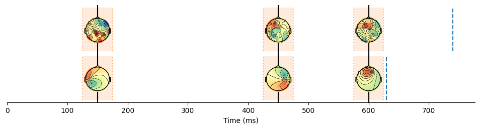
In this case we do indeed recover the correct events, quite close to the ground truth. The first two events are estimated separately for A and B, while the third event is shared across both participants which does help the model to get the correct amplitude and time for the third event.