3. Applying HMP to real data#

For this tutorial we will use the data from application 2 of this this paper. For the purpose of this tutorial we will only use the first 5 participants of the data (see the HMP paper for the method and GWeindel/man_hmp for the whole (preprocessed) data).

In this experiment, participants performed a random-dot motion task. They were asked to indicate the direction of motion of a cloud of moving dots. While a proportion of the dots moved in a target direction, the remainder moved randomly and makes the direction discrimination more difficult. Difficulty of the task was calibrated per subject. Prior to each trial, participants received a cue that indicated whether they should respond as quickly as possible or whether they should focus on giving an accurate response: the ‘speed’ and ‘accuracy’ conditions. In this tutorial we will ignore the difference between these conditions, but in the next tutorial we will look at how we can take conditions into account in the HMP analysis.

Fitting#

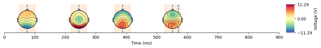
As introduced in Tutorial 2, the CumulativeEstimation method starts by sliding a candidate event from 0 to mean RT. When an event is found – the Expectation Maximization estimation converges – one event is added to the model and the slide continues. This way we can detect new events while accounting for the previous ones.

[6]:

model = hmp.models.CumulativeMethod(event_properties)
_, estimates_cumulative = model.fit_transform(trial_data)

1 events found around times [83]
2 events found around times [86, 280]
3 events found around times [86, 276, 503]
4 events found around times [83, 263, 440, 693]
Found 4 events

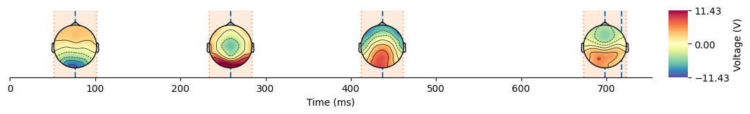
[7]:

hmp.visu.plot_topo_timecourse(epoch_data, estimates_cumulative, info, as_time=True)

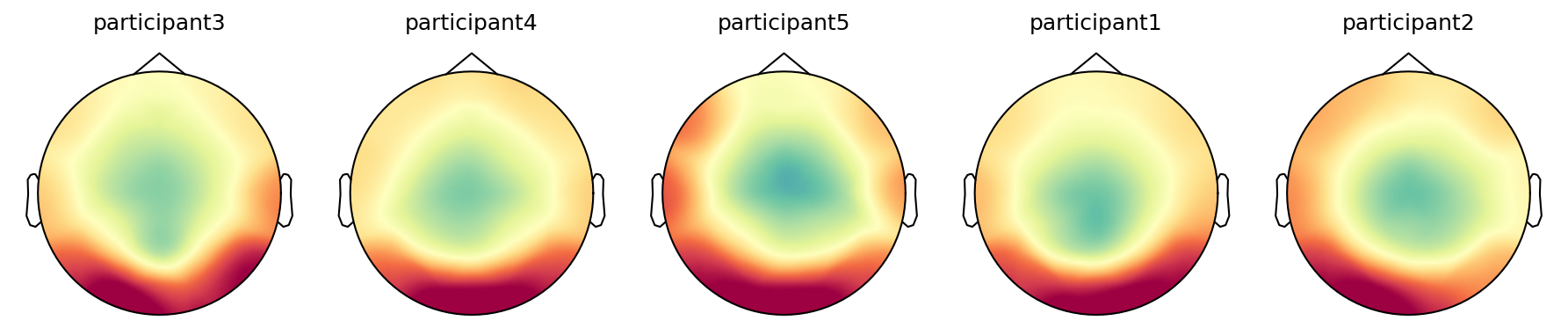
../_images/notebooks_3-Applying_HMP_to_real_data_16_0.png

Example application 1: looking at individual topographies#

[8]:

# Plotting individual topographies for a specific event across participants
from mne.viz import plot_topomap

# Get event-channel weights for each trial
by_trial_weights = hmp.utils.event_channels(epoch_data, estimates_cumulative, mean=False)

# Plot topographies for each participant for a selected event
fig, axes = plt.subplots(1, 5, dpi=150, figsize=(12, 2.5))
axes = axes.flatten()
event = 2 # Event index to plot (1-based for display, 0-based for indexing)

# Looking at the topographies of the 5 first participants
for i, participant in enumerate(epoch_data.participant[:5]):
    ax = axes[i]
    # Average across epochs for the selected event and participant
    topo = by_trial_weights.sel(event=event-1, participant=participant).mean('epoch')
    plot_topomap(
        topo,
        info,
        sensors=False,
        cmap='Spectral_r',
        res=100,
        show=False,
        axes=ax,
        contours=False
    )
    ax.set_title(f'{str(participant.values)[:-4]}')

plt.tight_layout()

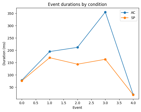
../_images/notebooks_3-Applying_HMP_to_real_data_18_0.png

Example application 2: analyzing condition effect on interval between events#

[9]:

# Compute max likely time for each trial and each event
times =  hmp.utils.event_times(estimates_cumulative, duration=True, add_rt=True, as_time=True)
times

[10]:

# Turn into dataframe and recover metadata
times = times.unstack().to_dataframe(name='duration')
times = times[~times.duration.isna()]  #Remove rejected trials
times = times.reset_index().set_index(['participant','epoch'])

# Recover metadata and merge with times
times_metadata = epoch_data.sel(sample=0, channel='Cz').to_dataframe().iloc[:,3:]
times_metadata = times_metadata.reset_index().set_index(['participant','epoch'])
times = times.merge(times_metadata, on=['participant','epoch'])

times

[10]:

		event	group	duration	stim	resp	RT	cue	movement	trigger
participant	epoch
participant1_epo	1	0	0.0	156.666667	1.0	resp_left	683.0	SP	stim_left	SP/stim_left/resp_left
	2	0	0.0	33.333333	1.0	resp_right	1068.0	AC	stim_left	AC/stim_left/resp_right
	3	0	0.0	20.000000	1.0	resp_right	994.0	SP	stim_left	SP/stim_left/resp_right
	4	0	0.0	173.333333	1.0	resp_left	1352.0	AC	stim_left	AC/stim_left/resp_left
	5	0	0.0	96.666667	2.0	resp_left	722.0	SP	stim_right	SP/stim_right/resp_left
...	...	...	...	...	...	...	...	...	...	...
participant5_epo	193	4	0.0	16.666667	1.0	resp_right	555.0	AC	stim_left	AC/stim_left/resp_right
	194	4	0.0	13.333333	1.0	resp_left	418.0	AC	stim_left	AC/stim_left/resp_left
	195	4	0.0	16.666667	1.0	resp_right	377.0	SP	stim_left	SP/stim_left/resp_right
	197	4	0.0	20.000000	1.0	resp_right	649.0	AC	stim_left	AC/stim_left/resp_right
	199	4	0.0	20.000000	1.0	resp_right	301.0	AC	stim_left	AC/stim_left/resp_right

4500 rows × 9 columns

[11]:

mean_ac = times[times.cue == 'AC'].groupby(['event']).duration.mean()
mean_sp = times[times.cue == 'SP'].groupby(['event']).duration.mean()

plt.plot(mean_ac.index, mean_ac.values, 'o-', label='AC')
plt.plot(mean_sp.index, mean_sp.values, 'o-', label='SP')
plt.legend()
plt.xlabel('Event')
plt.ylabel('Duration (ms)')
plt.title('Event durations by condition')

[11]:

Text(0.5, 1.0, 'Event durations by condition')

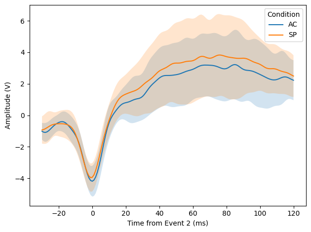
../_images/notebooks_3-Applying_HMP_to_real_data_22_1.png

Example application 3: Comparing conditions on centered ERPs:#

[12]:

# Plotting centered ERPs for each condition (AC and SP) with confidence intervals (±1 std)
fig, ax = plt.subplots(1,1)

# Get event times (positions not durations) for all events/trials, including stimulus onset
times_position = hmp.utils.event_times(estimates_cumulative, duration=False, mean=False, add_stim=True)

# Define window size in samples
baseline = -.1*sfreq  # 100 ms before event
n_samples = .4*sfreq  # 400 ms window

event = 2  # Event index to center on, 0 is stimulus

# Select a subset of channels to analyze (e.g., centroparietal channels)
channel_subset = ['CP1', 'CP2']

for SAT in ["AC","SP"]:
    # Select trials for the current condition and stack participant/epoch as 'trial' for easiness
    subset = epoch_data.where((epoch_data.cue == SAT), drop=True).stack({'trial':['participant','epoch']}).data.dropna('trial', how="all")
    # Center activity on the event for selected channels
    centered = hmp.utils.centered_activity(subset, times_position, channel_subset,
        event=event, n_samples=n_samples, baseline=baseline)
    # Average across channels,
    centered = centered.data.unstack().mean('channel')
    # Compute mean and std across participants
    indiv_traces = centered.groupby('participant').mean(dim='epoch')
    mean_tc = indiv_traces.mean('participant')
    std_tc = indiv_traces.std('participant')
    # Plot the timecourse with confidence interval
    ax.plot(centered.sample, mean_tc, label=SAT,)
    ax.fill_between(centered.sample, mean_tc-std_tc, mean_tc+std_tc, alpha=0.2)
ax.set_xlabel(f'Time from Event {event} (ms)')
ax.set_ylabel('Amplitude (V)')
plt.legend(title='Condition')
plt.tight_layout()

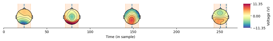
../_images/notebooks_3-Applying_HMP_to_real_data_24_0.png

Splitting conditions#

When estimating a model across all conditions, we can also split the data by condition. This is useful to see how the model estimates differ across conditions, such as speed vs accuracy instructions in this case.

[13]:

speed_epoch_data = epoch_data.where(epoch_data.cue == 'SP').stack({'trial':['participant','epoch']}).dropna('trial', how="all")
accuracy_epoch_data = epoch_data.where(epoch_data.cue == 'AC').stack({'trial':['participant','epoch']}).dropna('trial', how="all")

hmp.visu.plot_topo_timecourse(speed_epoch_data, estimates_cumulative, info, as_time=True, max_time=900)
hmp.visu.plot_topo_timecourse(accuracy_epoch_data, estimates_cumulative, info, as_time=True, max_time=900)

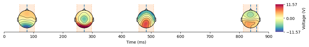
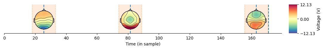
../_images/notebooks_3-Applying_HMP_to_real_data_27_0.png

../_images/notebooks_3-Applying_HMP_to_real_data_27_1.png

But in this case the HMP parameters are all shared across conditions so we might want to estimate the model separately for each condition if there is a reason to expect a difference. This is done by selecting the condition of interest and then estimating the model on the selected data.

[14]:

speed_preprocessed_data = hmp.utils.condition_selection(preprocessed.data, 'SP', variable='cue')
trial_data_speed = hmp.trialdata.TrialData.from_transformer(speed_preprocessed_data, pattern=event_properties.template)

accuracy_preprocesssed_data = hmp.utils.condition_selection(preprocessed.data, 'AC', variable='cue')
trial_data_accuracy = hmp.trialdata.TrialData.from_transformer(accuracy_preprocesssed_data, pattern=event_properties.template)

[15]:

model_speed = hmp.models.CumulativeMethod(event_properties)
model_speed.fit(trial_data_speed)
ll_cumulative_speed, estimates_speed = model_speed.transform(trial_data_speed)
hmp.visu.plot_topo_timecourse(epoch_data, estimates_speed, info)

1 events found around times [93]
2 events found around times [93, 280]
3 events found around times [90, 276, 536]
Found 3 events

../_images/notebooks_3-Applying_HMP_to_real_data_30_2.png

[16]:

model_accuracy = hmp.models.CumulativeMethod(event_properties)
model_accuracy.fit(trial_data_accuracy)
ll_cumulative_accuracy, estimates_accuracy = model_accuracy.transform(trial_data_accuracy)
hmp.visu.plot_topo_timecourse(epoch_data, estimates_accuracy, info)

1 events found around times [83]
2 events found around times [86, 283]
3 events found around times [86, 276, 523]
4 events found around times [86, 273, 503, 826]
Found 4 events

../_images/notebooks_3-Applying_HMP_to_real_data_31_2.png

In this case, the models are completely independent and the cumulative method finds an additional event for the accuracy condition, but not for the speed condition.

In the next advanced tutorials we cover how to build models that share some parameters between conditions or participants.